Algorithmic Audio Feature Extraction in English

High-level summary: how to get pretty graphs, nice numbers, and Python code to accurately describe sounds.

05/25/2020 5:34 PM update: I have yet to proofread this and organize the Essentia versus LibROSA code examples. It's a lot. I'll get it done. For now, just bear with me.

In order to make machines intelligent like humans, we often rely on machine learning and artificial intelligence techniques. There are several reasons why we want computers to be able to make human-like decisions. Developing smarter artificial agents and studying our interaction with them serve as an intermediary for better understanding human behavior and cognition.

Contents

1. Time domain features: windowing techniques, zero-crossing rate (ZCR), characterizing energy using short time energy (STE) and root mean square energy (RMSE), separating harmonic & percussive signals, and beat extraction.
2. Frequency domain features: chroma-related features, tonality based features
3. Spectrum shape based features: spectral centroids, spectral contrast, spectral rolloff, and mel-frequency cepstral coefficients (MFCCs)
4. Using features for analysis: hum, discontinuity, and click detection algorithms

Despite extensive research on vision, emotion, and cognition, modeling the human auditory system in machines remains understudied. If our machines could hear as well as humans do, we would expect them to easily distinguish speech from music or ambient noises, to know what direction sounds are coming from, to accurately enumerate the number of sound-producing objects in the room, to differentiate between sounds that are typical and those that are noteworthy, and to effortlessly characterize important features of any given audio source. Such machines should also be able to organize what they hear, learn names for recognizable objects and styles, and retrieve memory of a sound by reference to a handful of descriptors. These machines should be able to listen and react in real time, to take appropriate action to respond to having heard a noteworthy event.

These abilities present unique challenges to computer scientists (to build better machines) and psychologists (to better understand these human functions), and are collectively motivations for the emerging field of machine hearing. Regardless of any one aim, a machine requires a set of robust and discriminatory features to accurately and quickly achieve its goal. For an ML system (and arguably also for a human child), intelligence is defined by the amount and quality of training given to it. It is typical for one to reduce the size representation of the signals used to train the machine as opposed to feeding it a complete dataset. Compact representations of a signal, also called features, reduce the size of the orginal signal signficantly while still describing the signal completely and accurately. As a result, the reduced representation improves the computational and time complexities of the ML algorithm, making it more suitable for real-time applications.

Audio feature extraction

Feature extraction is the process of highlighting the most discriminating and impactful features of a signal. The evolution of features used in audio signal processing algorithms begins with features extracted in the time domain (< 1950s), which continue to play an important role in audio analysis and classification. Analyzing the spectrum for several features such as pitch, formants, etc. originates from the frequency domain (< 1960s). Eventually, joint time-frequency techniques (> 1970s) allowed for analyzing signals in both the time and frequency domains simultaneously. Since the development of deep learning (> 2000s), deep features are extensively used in a diverse array of applications such as acoustic scene classification [1] and speaker recognition [2].

The remainder of this article will a walkthrough on extracting some of these features using the Essentia and LibROSA Python libraries. It will also be an attempt of an applied computer science student to explain what she's learned about signal processing theory in the past 48 hours. Enjoy.

Time domain features

%matplotlib inline  
import librosa                     # librosa music package
import essentia                    # essentia music package
import essentia.standard           # essentia for imperative programming
import essentia.streaming          # essentia for declarative programming

import IPython                     # for playing audio
import numpy as np                 # for handling large arrays
import pandas as pd                # for data manipulation and analysis
import scipy                       # for common math functions
import sklearn                     # a machine learning library
import os                          # for accessing local files

import librosa.display             # librosa plot functions
import matplotlib.pyplot as plt    # plotting with Matlab functionality
import seaborn as sns              # data visualization based on matplotlib

# in libROSA
audio_librosa = 'audio/human-rights.wav' # audio file path
y, sr = librosa.core.load(audio_librosa) # load samples and determine sampling rate

# in Essentia
loader = essentia.standard.MonoLoader(filename='audio/human-rights.wav') # instantiate audio loader
audio_essentia = loader() # actually load audio file

# to hear how the audio we want to process sounds like
IPython.display.Audio('audio/human-rights.wav')

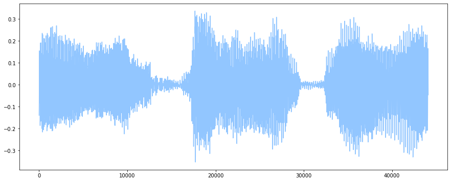
plt.rcParams['figure.figsize'] = (15, 6) # instantiate plot canvas
plot(audio[1*44100:2*44100]) # get the 2nd second of the audio clip
show()

Windowing in time domain

Before we discuss time domain features, it is necessary to introduce the concept of windowing in time domain. The simplest way to analyze a signal is in its raw form. For time series signals (signals that evolve with time), windowing allows us to view a short time segment of a longer signal and analyze its frequency content. Mathematically, windowing can be seen as multiplying a signal with a window function that is zero everywhere on the given signal except on the region of interest. The simplest type of window is a rectangular window such as that defined by $$W(n) = \left\{ \begin{array}{ll} 1, & -\frac{M-1}{2} \leq n \leq \frac{M-1}{2} \\ 0, & otherwise \end{array} \right.$$

As the window slides over the signal in time, the size is made adaptive by changing according to characteristics of the audio signal. One problem with this is the abrupt changes or jump discontinuities in its shape at the edges of the window. The distortion is the result of the Gibbs phenomenon. To solve this, we can use a window function with smooth curves like the Hann function: $$\left.\begin{array}{rl} W(n)=w_{0}\left(\frac{L}{N}(n-N / 2)\right) & =\frac{1}{2}\left[1-\cos \left(\frac{2 \pi n}{N}\right)\right] \\ & =\sin ^{2}\left(\frac{\pi n}{N}\right) \end{array}\right\}, \quad 0 \leq n \leq N,$$ where the length of the window is \(N + 1\). In summary, these functions round the corners of rectangular windows to downgrade the edge of the signal, reducing the edge effect and therefore the Gibbs phenomenon.

w_essentia = Windowing(type = 'hann')    # specify window function in essentia
w_scipy = signal.get_window('triang', 7) # apply window function in scipy
w_librosa= signal.get_window('hamm', 7)  # apply window function in librosa 

The windowing method in LibROSA is provided as a wrapper for the scipy function of the same name that also supports callable or pre-computed windows. For a list of window types supported by scipy and LibROSA, see scipy.signal.get_window. For a list of types supported by Essentia, see essentia.standard.Windowing.

Zero-crossing rate (ZCR)

The ZCR of an audio grame is defined as the rate at which the signal changes sign. ZCR is an efficient and simple way to detecting whether a speech frame is voice, unvoiced, or silent. It is expected that unvoiced segments produce higher ZCRs than for voice segments, and ideally ZCRs equal to zero for silence segments [3].

ZCR is also an essential technique for estimating fundamental frequency, the lowest frequency of a periodic waveform. The ZCR feature can therefore be used to design discriminator and classifier systems. With this additional information, this feature demonstrates, for example, a higher ZCR for music sources than for speech source. To see the implementation of such a system, check out "A speech/music discriminator based on RMS and zero-crossings."

# SETUP
w = Windowing(type = 'hann')    # state windowing function
spectrum = Spectrum()           # instead of a complex FTT (the output of FFT()), we just want the magnitude spectrum
zcr = ZeroCrossingRate()        # instantiate the essentia.standard zero-crossing function

zcrs = []
frameSize = 1024
hopSize = 512

# APPLY ZCR FUNCTION to SPEECH signal

# iterating through frames matlab style:
# for fstart in range(0, len(audio)-frameSize, hopSize):
#   frame = audio[fstart:fstart+frameSize]

# iterating through frames essentia style:
for frame in FrameGenerator(audio, frameSize=1024, hopSize=512, startFromZero=True):
    zcrs.append(zcr(spectrum(w(frame))))

zcrs = essentia.array(zcrs).T # shape output array

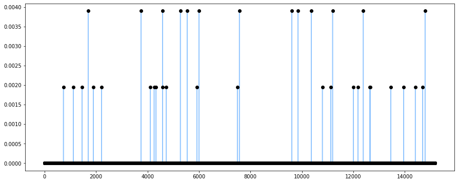
# PLOT OUTPUT
zcrs_x = range(0, len(zcrs))
zcrs_y = zcrs
plt.plot(zcrs_x, zcrs_y, 'o', color='black') # plot ZCR per frame as points
plt.plot(zcrs) # plot time-series change in ZCRs
show()

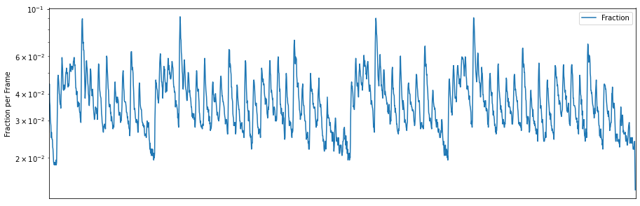
# APPLY LibROSA ZCR FUNCTION to MUSIC signal
zcr = librosa.feature.zero_crossing_rate(y) 

# PLOT OUTPUT
plt.figure(figsize=(15,5))
plt.semilogy(zcr.T, label='Fraction') # apply log transform on y
plt.ylabel('Fraction per Frame')
plt.xticks([])
plt.xlim([0, rolloff.shape[-1]])
plt.legend()    

Characterizing Energy

The sound signals here are non-stationary time series which means that its statistical properties (e.g., mean, variance) are changing over time. A stationary time series has constant statistical properties. Non-stationary signals must be first converted into stationary data before performing further analysis (to avoid under/over-estimating the mean and variance). This conversion can be achieved, for example, by trend removal which involves fitting the series to a regression line and then subtracting it from the original signal, or using framing/windowing methods as previously discussed to transform small chunks of the non-stationary signal into quasi-stationary signals.

The energy of a signal corresponds to its total magnitude. For audio signals this roughly characterizes how loud the signal is. Two methods for individually characterizing signal energy are short time energy and root mean square energy measures.

Short Time Energy (STE)

The energy throughout a raw sound signal is variable and it is difficult, therefore, to accurately characterize the energy of a signal. For this, the short time energy, which is the energy from a frame, is calculated. With similar applications to ZCRs, STE is used to detect voiced-unvoiced segments, aid in music onset detection, and discriminate between source types (music, environmental, speech).

def calculateSTE(audio_signal, window_type, frame_length, hop_size):
    signal_new = []                           # container for signal square
    win = Windowing(type = window_type)       # instantiate window function
    
    # compute signal square by frame
    for frame in FrameGenerator(audio_signal, frameSize=frame_length, hopSize=hop_size, startFromZero=True):
        frame_new = frame**2
        signal_new.append(frame_new)
    
    # output the convolution of window and signal square
    return np.convolve(signal_new, win)

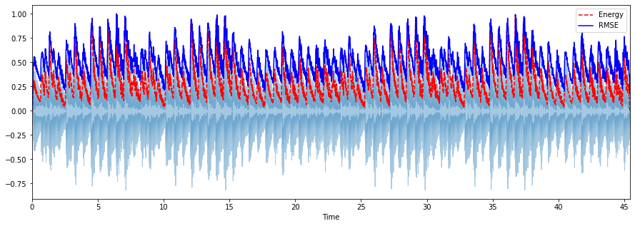
Root Mean Square Energy (RMSE)

The RMSE of a signal follows a similar calculation as the STE method, where RSME is instead the squart root of the mean square (the average of the squares of magnitude of the audio frames).

hop_length = 256
frame_length = 512
    
# compute sum of signal square by frame
energy = np.array([
    sum(abs(y[i:i+frame_length]**2))
    for i in range(0, len(y), hop_length)
])
energy.shape

# compute RMSE over frames
rmse = librosa.feature.rms(y, frame_length=frame_length, hop_length=hop_length, center=True)
rmse.shape
rmse = rmse[0]

# plot energy and rmse along the waveform
frames = range(len(energy))
t = librosa.frames_to_time(frames, sr=sr, hop_length=hop_length)

plt.figure(figsize=(15, 5))
librosa.display.waveplot(y, sr=sr, alpha=0.4)
plt.plot(t, energy/energy.max(), 'r--')                # normalized for visualization
plt.plot(t[:len(rmse)], rmse/rmse.max(), color='blue') # normalized for visualization
plt.legend(('Energy', 'RMSE'))

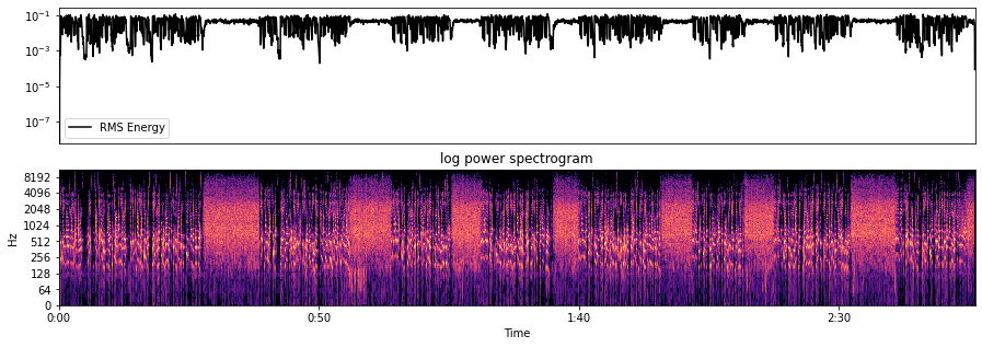
Computing the RMS value from audio samples is faster than alternative energy calculations requiring short-time Fourier transform (STFT) calculations. STFTs are used to determine the sinusoidal frequency and phase content of portions of the signal over time. After dividing the raw signal into quasi-stationary segments, to compute STFTs is to perform the Fourier transform (which simply decomposes a signal into its constituent frequencies) on each segment.

However, using a spectrogram, a visual representation of the spectrum of frequencies over time, can give us a more accurate representation of energy because its frames can be windowed. Therefore, if a spectrogram is already available, we prefer to run the RMS function over it:

S, phase = librosa.magphase(librosa.stft(y)) # compute magnitude and phase content
rms = librosa.feature.rms(S=S) # compute root-mean-square for each frame in magnitude

plt.figure(figsize=(15, 5))
plt.subplot(2, 1, 1)
plt.semilogy(rms.T, label='RMS Energy', color="black")
plt.xticks([])
plt.xlim([0, rms.shape[-1]])
plt.legend()
plt.subplot(2, 1, 2)
librosa.display.specshow(librosa.amplitude_to_db(S, ref=np.max),
                            y_axis='log', x_axis='time')
plt.title('log power spectrogram')

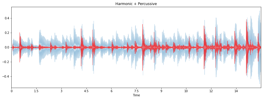
Separation of Harmonic & Percussive Signals

On a very coarse level, many sounds can be categorized as either of the harmonic or percussive sound class. Harmonic sounds are sounds we perceive to have a specific pitch, whereas percussive sounds are often perceived as the result of two colliding objects. Percussive sounds tend to have a clear localization in time moreso than a particular pitch. More granular sound classes can be classified by its harmonic-percussive components ratio. For example, a note played on the piano has a percussive onset (marked by the hammer hitting the strings) preceding a harmonic tone (the result of the vibrating string).

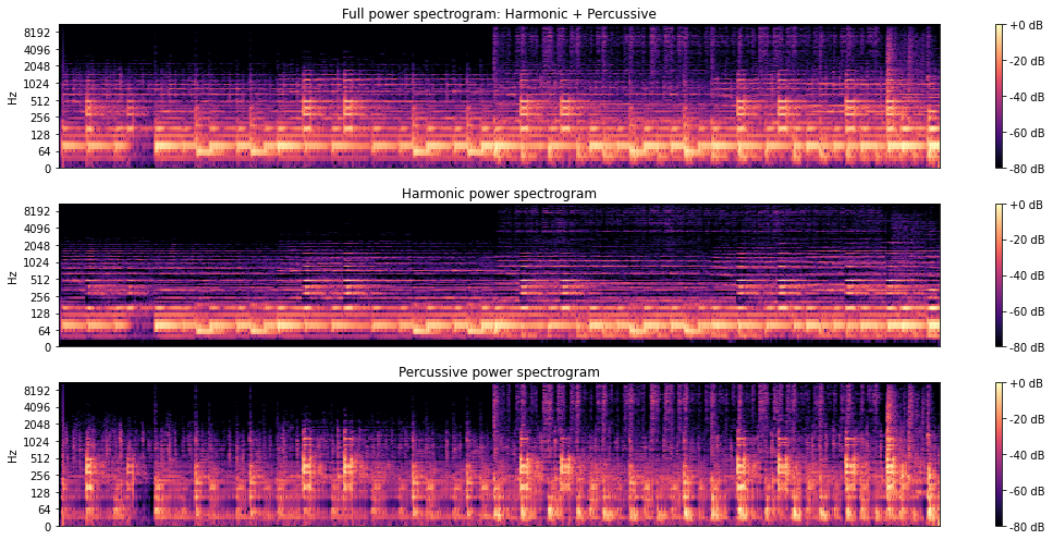
The value of mapping both the time and phase content of a signal in distinguishing between harmonic and percussive components, makes the STFT spectral representation important. The time-frequency bin of the STFT for harmonic component of an input signal is expected to look more horizontal than vertical/time-dependent structure that is a percussive component. Applying this harmonic-percussive source separation algorithm without explicit intermediary analysis of the STFT spectrum looks like this:

y_harmonic, y_percussive = librosa.effects.hpss(y)

plt.figure(figsize=(15, 5))
librosa.display.waveplot(y_harmonic, sr=sr, alpha=0.25)
librosa.display.waveplot(y_percussive, sr=sr, color='red', alpha=0.5)
plt.title('Harmonic + Percussive')
plt.show()

# showing differences in STFT representations
y, sr = librosa.load(librosa.util.example_audio_file(), duration=15)
D = librosa.stft(y)
H, P = librosa.decompose.hpss(D)
    
plt.figure(figsize=(15, 7))
plt.subplot(3, 1, 1)
librosa.display.specshow(librosa.amplitude_to_db(np.abs(D), ref=np.max), y_axis='log')
plt.colorbar(format='%+2.0f dB')
plt.title('Full power spectrogram: Harmonic + Percussive')

# harmonic spectrogram will show more horizontal/pitch-dependent changes
plt.subplot(3, 1, 2)
librosa.display.specshow(librosa.amplitude_to_db(np.abs(H), ref=np.max), y_axis='log')
plt.colorbar(format='%+2.0f dB')
plt.title('Harmonic power spectrogram')
plt.subplot(3, 1, 3)

# percussive spectrogram will show more vertical/time-dependent changes
librosa.display.specshow(librosa.amplitude_to_db(np.abs(P), ref=np.max), y_axis='log')
plt.colorbar(format='%+2.0f dB')
plt.title('Percussive power spectrogram')
plt.tight_layout()
plt.show()

Beat Extraction

Particularly useful features to extract from musical sources may be an approximation of tempo as well as the beat onset indices, an array of frame numbers corresponding to beat events:

tempo, beat_frames = librosa.beat.beat_track(y=y_harmonic, sr=sr)

print('Detected Tempo: '+ str(tempo) + ' beats/min')
beat_times = librosa.frames_to_time(beat_frames, sr=sr)
beat_time_diff = np.ediff1d(beat_times)
beat_nums = np.arange(1, np.size(beat_times))

fig, ax = plt.subplots()
fig.set_size_inches(15, 5)
ax.set_ylabel("Time difference (s)")
ax.set_xlabel("Beats")
g = sns.barplot(beat_nums, beat_time_diff, palette="rocket",ax=ax)
g = g.set(xticklabels=[])

Detected Tempo: 161.4990234375 beats/min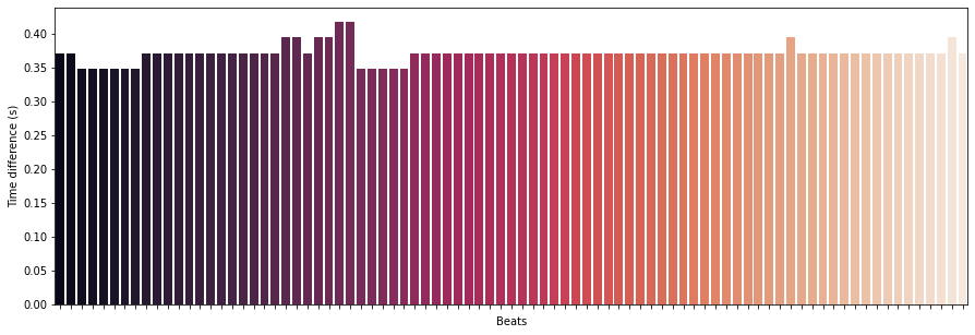

Frequency domain features

Time-domain plots show signal variation with respect to time. Therefore, to analyze a signal in terms of frequency, the time-domain signal is converted into frequency-domain signals using transforms such as the Fourier transform or auto-regression analysis. We've already seen this implemented in previous time-domain feature extraction using STFTs.

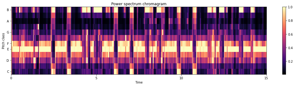
Chroma related features

Chroma features are a powerful representation of music audio in which we use a 12-element representation of spectral energy called a chroma vector where each of the 12 bins represeent the 12 equal-tempered pitch class of western-type music (semitone spacing). It can be computed from the logarithmic short-time Fourier transform of the input sound signal, also called a chromagram or a pitch class profile.

# using a power spectrum
chroma_d = librosa.feature.chroma_stft(y=y, sr=sr)

plt.figure(figsize=(15, 4))
librosa.display.specshow(chroma_d, y_axis='chroma', x_axis='time')
plt.colorbar()
plt.title('Power spectrum chromagram')
plt.tight_layout()
plt.show()

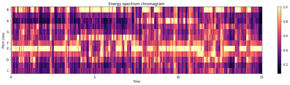
# using an energy (magnitude) spectrum
S = np.abs(librosa.stft(y)) # apply short-time fourier transform
chroma_e = librosa.feature.chroma_stft(S=S, sr=sr)

plt.figure(figsize=(15, 4))
librosa.display.specshow(chroma_e, y_axis='chroma', x_axis='time')
plt.colorbar()
plt.title('Energy spectrum chromagram')
plt.tight_layout()
plt.show()

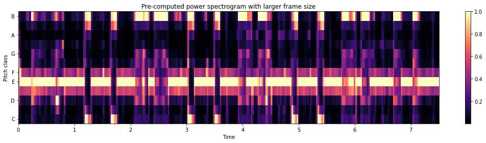
# using a pre-computed power spectrogram with a larger frame
S = np.abs(librosa.stft(y, n_fft=4096))**2
chroma_p = librosa.feature.chroma_stft(S=S, sr=sr)

plt.figure(figsize=(15, 4))
librosa.display.specshow(chroma_p, y_axis='chroma', x_axis='time')
plt.colorbar()
plt.title('Pre-computed power spectrogram with larger frame size')
plt.tight_layout()
plt.show()

Another chroma-based feature is chroma energy distribution normalized statistics (CENS) which is typically used to identify similarity between different interpretations of the music given. The main idea of CENS is that taking statistics over large windows of an audio file smooths local deviations in tempo, articulation, and musical ornaments. CENS are typically implemented for audio matching and similarity tasks.

chroma = librosa.feature.chroma_cens(y=y_harmonic, sr=sr)
plt.figure(figsize=(15, 4))
librosa.display.specshow(chroma,y_axis='chroma', x_axis='time')
plt.colorbar()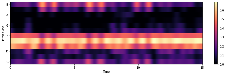

Tonality-based features

The tonal sounds of a harmonic stationary audio signal is actually the fundamental frequency (FF). The more technical definition of the FF is that it is the first peak of the local normalized spectrotemporal auto-correlation function (english translation: the lowest frequency of a periodic waveform). FF is an important feature for music onset detection, audio retrieval, and sound type classification.

# psuedocode for FF detection
1. Input: audio signal x and sampling frequency sf
2. Find the pitch of an audio signal by auto-correlation or cepstral methods
3. Return pitch, an estimate of the FF of x

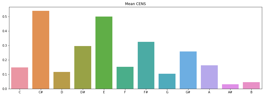
Other tonality-based features include pitch histograms which explain the pitch of a signal in a more compact form, pitch profiles, harmonicity which distinguishes between tonal- and noise-like sounds by finding periodicity in sound in either the time or frequency domain, and harmonic-to-noise ratios.

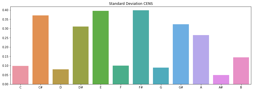
# a pitch histogram using CENS
chroma_mean = np.mean(chroma,axis=1)
chroma_std = np.std(chroma,axis=1)

# plot the summary
octave = ['C','C#','D','D#','E','F','F#','G','G#','A','A#','B']
plt.figure(figsize = (15,5))
plt.title('Mean CENS')
sns.barplot(x=octave,y=chroma_mean)

plt.figure(figsize = (15,5))
plt.title('Standard Deviation CENS')
sns.barplot(x=octave,y=chroma_std)

Spectrum shape based features

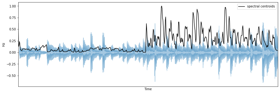
Spectral centroid

The spectral centroid is a measure to characterize the "center of mass" of a given spectrum. Perceptually, it has a robust connection with the impression of sound "brightness". Timbre researchers formalize brightness as an indication of the amount of high-frequency content in a sound.

The spectral centroid is calculated as the weighted means of the frequencies present in a given signal, determined using a Fourier transform, with the frequency magnitudes as the weights: \(centroid =\left(\sum_{k=b_{1}}^{b_{2}} f_{k} s_{k}\right) /\left(\sum_{k=b_{1}}^{b_{2}} s_{k}\right)\), where \(f_{k}\) is the frequency corresponding to bin \(k\) and \(s_{k}\) is the spectral value at bin \(k\), \(b_{1}\) and \(b_{2}\) are the band edges.

# compute the spectral centroid for each frame in a signal
spectral_centroids = librosa.feature.spectral_centroid(y=y, sr=sr)[0]
spectral_centroids.shape

# compute the time variable for visualization
frames = range(len(spectral_centroids))
f_times = librosa.frames_to_time(frames)

# an auxiliar function to normalize the spectral centroid for visualization
def normalize(x, axis=0):
    return sklearn.preprocessing.minmax_scale(x, axis=axis)

plt.figure(figsize=(15,5))
plt.subplot(1, 1, 1)
librosa.display.waveplot(y, sr=sr, alpha=0.4)
plt.plot(f_times, normalize(spectral_centroids), color='black', label='spectral centroids')
plt.ylabel('Hz')
plt.xticks([])
plt.legend()    

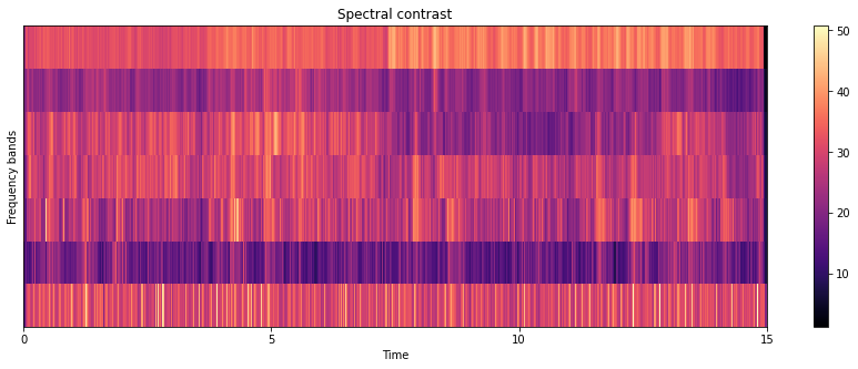
Spectral contrast

Octave-based Spectral Contrast (OSC) was developed to represent the spectral characteristics of a musical piece. It considers the spectral peak and valley in each sub-band separately.

# pseudocode of OSC extraction
1. Input: audio signal x
2. Perform windowing over the signal
3. Take FFT of each signal frame
4. Divide the transformed signal into 6 octave scaled sub-bands
5. For each band, calculate peak and valley values
6. Calculate the contrast of the peaks and valleys
7. Output contrast and valleys as the OSC feature set

In general, spectral peaks correspond to harmonic components and spectral valleys correspond to non-harmonic components or noise in a music piece. Therefore, the difference between spectral peaks and spectral valleys will reflect the spectral contrast distribution.

contrast = librosa.feature.spectral_contrast(y=y_harmonic,sr=sr)

plt.figure(figsize=(15,5))
librosa.display.specshow(contrast, x_axis='time')
plt.colorbar()
plt.ylabel('Frequency bands')
plt.title('Spectral contrast')

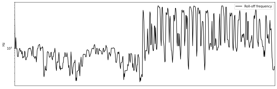
Spectral Rolloff

Spectral rolloff point is defined as the \(N\)th percentile frequency of the power spectral distribution, where \(N\) is usually 85% or 95%. The rolloff point is the frequency below which the \(N\)% of the magnitude distribution is concentrated. In other words, the spectral rolloff point is the frequency so the \(N%\) of the signal energy is contained below the this frequency. Mathematically, this is represented as \(rolloff = \sum_{k=b_{1}}^{d} s_{k}=N\left(\sum_{k=b_{1}}^{b_{2}} s_{k}\right)\), where \(s_{k}\) is the spectral value at bin \(k\), \(N\) is the percentile cutoff, and \(b_{1}\) and \(b_{2}\) are the band edges.

This measure is useful in distinguishing voiced speech from unvoiced: unvoiced speech has a high proportion of energy contained in the high-frequency range of the spectrum, where most of the energy for voiced speech and music is contained in lower bands.

rolloff = librosa.feature.spectral_rolloff(y=y, sr=sr)

plt.figure(figsize=(15,5))
plt.semilogy(rolloff.T, label='Roll-off frequency')
plt.ylabel('Hz')
plt.xticks([])
plt.xlim([0, rolloff.shape[-1]])
plt.legend()    

rolloff_mean = np.mean(rolloff)
rolloff_std = np.std(rolloff)
rolloff_skew = scipy.stats.skew(rolloff,axis = 1)[0]
print('Mean: ' + str(rolloff_mean))
print('STD: ' + str(rolloff_std))
print('Skewness: ' + str(rolloff_skew))    

Mean: 1548.2560100760093
SD: 1723.177533529806
Skewness: 1.6971059924278158

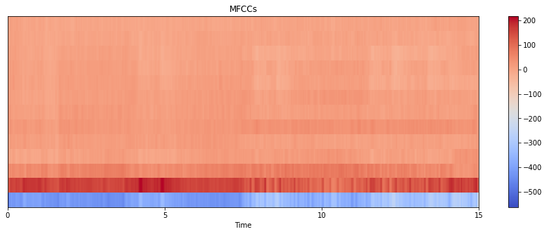
Mel-frequency cepstral coefficients (MFCCs)

A cepstrum is derived from taking the inverse Fourier transform of the logarithm of the raw signal spectrum. There are complex, power, phase, and real cepstrum representations. Among these, the power cepstrum proves to be the most relevant for speech signal processing. The analysis of the cepstrum is called quefrency analysis (the naming is a physicist' inside-joke to drawing a direct parallel to frequency analysis in the spectrum domain) or liftering (a parallel to filtering in the spectrum domain). Cepstrum features can be used for pitch detection, and speech recognition and enhancement.

Mel-frequency cepstral coefficients represent the short-time power an audio clip based on the discrete cosine transform of the log power spectrum on a non-linear mel scale. The difference between a cepstrum and the mel-frequency cepstrum (MFC) is that in the MFC, the frequency bands are equally spaced on the mel scale to more closely resemble the human auditory system's response as opposed to the linearly-spaced bands in the normal spectrum. This frequency warping allows for better representation of sound and is especially useful in audio compression.

# pseudocode for MFCC extraction
1. Input: audio signal x
2. Apply windowing function over the signal
3. For each frame, calculate the spectral density (periodogram) estimate of the power spectrum
4. Apply the mel-filter bank to the power spectrum 
5. Sum the energy in each filter 
6. Take the log of filter-bank energies
7. Take the discrete cosine transform (DCT) of the log filter-bank energies
8. Return the first 2-13 DCT coefficients, discarding the rest

mfccs = librosa.feature.mfcc(y=y_harmonic, sr=sr, n_mfcc=13)

plt.figure(figsize=(15, 5))
librosa.display.specshow(mfccs, x_axis='time')
plt.colorbar()
plt.title('MFCCs')    

Using features for analysis

Obviously we haven't covered all relevant audio features and how to extract each. However, this overview of the basic features allows us to perform more complex analyses.

# importing dependencies
import essentia.standard as es
import numpy as np
import matplotlib.pyplot as plt
from essentia import Pool
from essentia import db2amp
from IPython.display import Audio    

# an auxiliar function for plotting spectrograms
def spectrogram(audio, frameSize=1024, hopSize=512, db=True):
eps = np.finfo(np.float32).eps
window = es.Windowing(size=frameSize)
spectrum = es.PowerSpectrum(size=frameSize)
pool = Pool()
for frame in es.FrameGenerator(audio, frameSize=frameSize, hopSize=hopSize, startFromZero=True):
    pool.add('spectrogram', spectrum(window(frame)))
    
if db:
    return 10 * np.log10(pool['spectrogram'].T + eps)
else:
    return pool['spectrogram'].T    

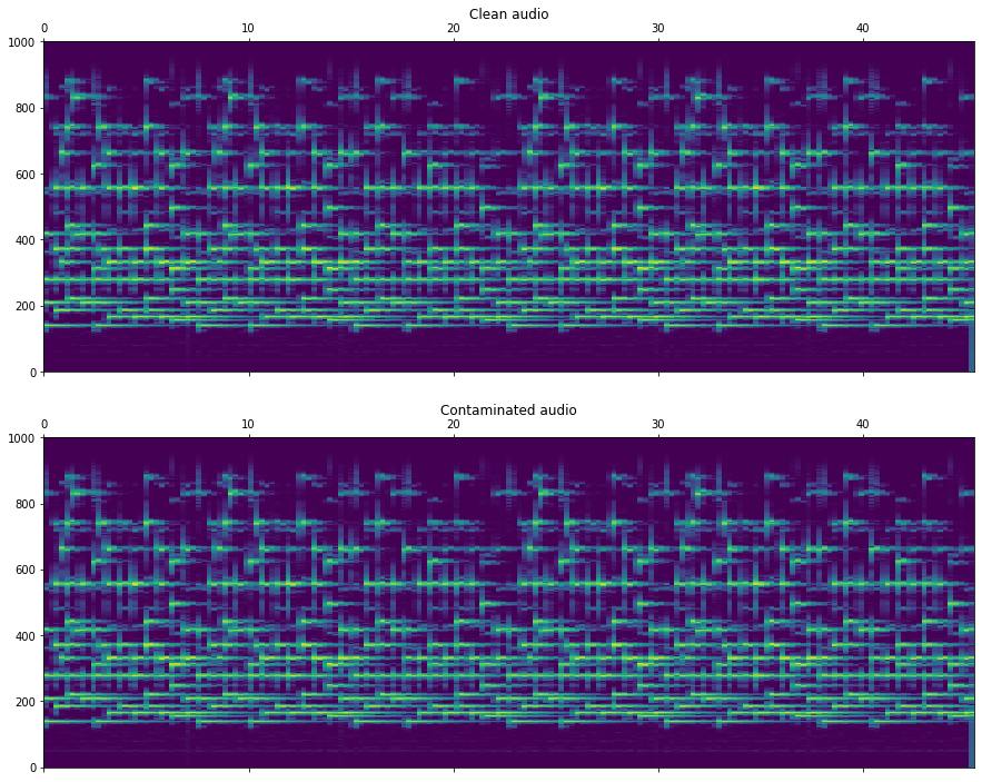
Hum detection

Audio files are sometimes contaminated with low-frequency humming tones degrading the audio quality. Typical causes for this problem are the electric installation frequency (aka mains hum; typically 50-60Hz) or poor electrical isolation on the recording or copying equipment. For the following example, we simulate this phenomenon by adding a 50Hz sinusoid with some harmonics.

This algorithm detects low frequency tonal noises in the audio signal. First, the steadiness of the power spectral density of the signal is computed by measuring the quantile ratios as described in [4]. Then, the essentia.streaming.PitchContours algorithm is used to track the humming tones. Check out "Modeling and analysis of Electric Network Frequency signal for timestamp verification" for a demonstrated implementation of hum detection in validating the authenticity of audio recordings using electrical network frequency analysis.

Generating an example signal

Let's downsample our audio gile to 2kHz as we are only interested in the lowest part of the spectrum.

file_name = '../../../test/audio/recorded/musicbox.wav'
audio = es.MonoLoader(filename=file_name)()
    
# downsampling
fs = 44100.
out_fs = 2000
audio_decimated = es.Resample(inputSampleRate=fs, outputSampleRate=out_fs)(audio)    

# generating the humming tone
nSamples = len(audio)
time = np.linspace(0, nSamples / 44100., nSamples)
freq = 50. # Hz
hum = 1.5 * np.sin(2 * np.pi * freq * time)

# adding some harmonics via clipping
hum = es.Clipper(min=-1., max=1.)(hum.astype(np.float32))

# adding some attenuation
hum *= db2amp(-36.)
audio_with_hum = np.array(audio + hum, dtype=np.float32)
audio_with_hum_decimated = es.Resample(inputSampleRate=fs, outputSampleRate=out_fs)(audio_with_hum)

# generate plots
fn = out_fs / 2.
f0 = 0.
f, ax = plt.subplots(2)

ax[0].matshow(spectrogram(audio_decimated), aspect='auto', origin='lower', extent=[0 , len(audio_decimated) / out_fs, f0, fn])
ax[0].set_title('Clean audio')

ax[1].matshow(spectrogram(audio_with_hum_decimated), aspect='auto', origin='lower', extent=[0 , len(audio_decimated) / out_fs, f0, fn])
ax[1].set_title('Contaminated audio')

Detection algorithm

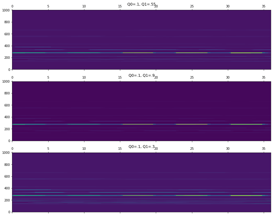
The detection algorithm relies on the fact that the humming tones are mostly constant on time. It measures the ratio between two quartiles of the power spectral density of the signal and expressess the results in a time versus frequency matrix where the peaks can be tracked. The following example illustrates the effect on choosing different quaratile parameters.

r0, _, _, _, _ = es.HumDetector(Q0=.1, Q1=.55)(audio_with_hum)
r1, _, _, _, _ = es.HumDetector(Q0=.1, Q1=.9)(audio_with_hum)
r2, _, _, _, _ = es.HumDetector(Q0=.1, Q1=.3)(audio_with_hum)

_, ax = plt.subplots(3)
f0 = 0
fn = 1000
ax[0].matshow(r0, aspect='auto', origin='lower', extent=[0 , r0.shape[1] * .2, f0, fn])
ax[0].set_title('Q0=.1, Q1=.55')

ax[1].matshow(r1, aspect='auto', origin='lower', extent=[0 , r1.shape[1] * .2, f0, fn])
ax[1].set_title('Q0=.1, Q1=.9')

ax[2].matshow(r2, aspect='auto', origin='lower', extent=[0 , r2.shape[1] * .2, f0, fn])
ax[2].set_title('Q0=.1, Q1=.3')

r0, freqs, saliences, starts, ends = es.HumDetector(Q0=.1, Q1=.55, detectionThreshold=5)(audio_with_hum)

plt.matshow(r0, aspect='auto', origin='lower', extent=[0 , r0.shape[1] * .2, f0, fn])
aLen = r0.shape[1] * .2
for i in range(len(freqs)):
    plt.axhline(y=freqs[i], xmin=starts[i] / aLen, xmax=ends[i] / aLen, alpha = saliences[i], color='r')
    
    print ('detected a {:.2f}Hz tone with salience {:.2f} starting at {:.2f}s and ending at {:.2f}s'\
            .format(freqs[i], saliences[i], starts[i], ends[i]))

detected a 275.60Hz tone with salience 0.27 starting at 10.00s and ending at 44.80s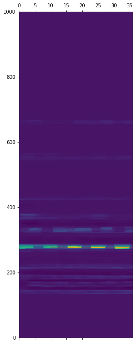

Relationship to sub-bass over-excitation

Hum detection is not beyond human hearing ability whereas sub-bass are more "felt" than "heard". Sub-bass over-excitation is not simply a phenomenon limited to a class of electronic speakers, but rather is a fundamental characteristic of all speakers regardless of quality or electrical interference. Sub-bass over-excitation would therefore give us a better measure of how "organic" an audio clip is [5].

Discontinuity detection

Discontinuities occur occasionally by hardware issues in the process of recording or copying. This algorithm described here uses Linear Predictive Coding and some heuristics as described in [6] to detect discontinuities in an audio signal.

# a stand-alone detector method
def compute(x, frame_size=1024, hop_size=512, **kwargs):
discontinuityDetector = es.DiscontinuityDetector(frameSize=frame_size, hopSize=hop_size, **kwargs)
locs = []
amps = []
for idx, frame in enumerate(es.FrameGenerator(x, frameSize=frame_size, hopSize=hop_size, startFromZero=True)):
    frame_locs, frame_ampls = discontinuityDetector(frame)

    for l in frame_locs:
        locs.append((l + hop_size * idx) / 44100.)
    for a in frame_ampls:
        amps.append(a)

return locs, amps

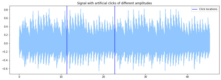
Generating an example signal

Let's start by degrading an audio file with some discontinuities by removing a random number of samples from the input audio file.

fs = 44100.
audio = es.MonoLoader(filename='../../../test/audio/recorded/musicbox.wav', sampleRate=fs)()

originalLen = len(audio)
startJumps = np.array([int(i) for i in [originalLen / 4, originalLen / 2]])
groundTruth = startJumps / float(fs)

for startJump in startJumps:
    # make sure that the artificial jump produces a prominent discontinuity
    if audio[startJump] > 0:
        end = next(idx for idx, i in enumerate(audio[startJump:]) if i < -.3)
    else:
        end = next(idx for idx, i in enumerate(audio[startJump:]) if i > .3)

    endJump = startJump + end
    audio = esarr(np.hstack([audio[:startJump], audio[endJump:]]))

times = np.linspace(0, len(audio) / fs, len(audio))
plt.plot(times, audio)
for point in groundTruth:
    l1 = plt.axvline(point, color='blue')
plt.title('Signal with artificial clicks of different amplitudes')
l1.set_label('Click locations')
plt.legend()    

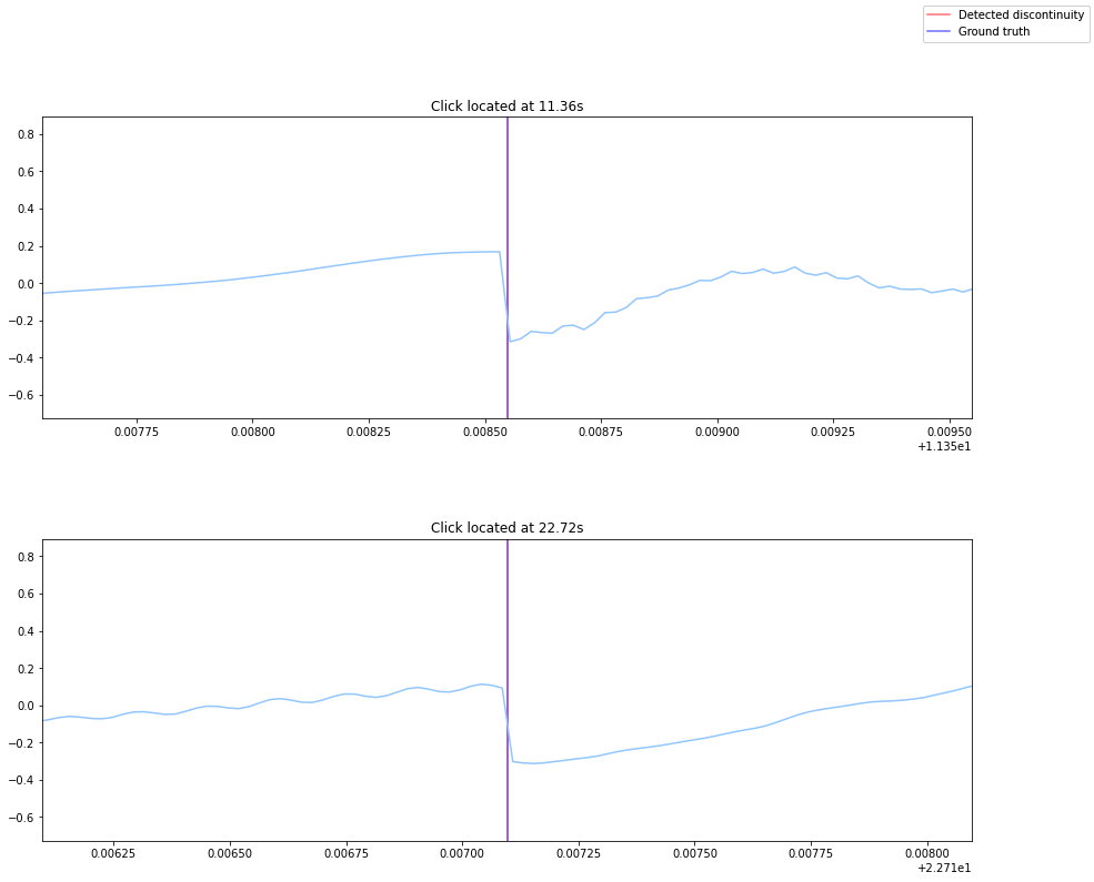
Detection algorithm

The algorithm should accurately determine the start and end timestamp of each click/discontinuity. The following plots show how the algorithm performs on the previously generated example audio.

locs, amps = compute(audio)

fig, ax = plt.subplots(len(groundTruth))
plt.subplots_adjust(hspace=.4)
for idx, point in enumerate(groundTruth):
    l1 = ax[idx].axvline(locs[idx], color='blue', alpha=.5)
    l2 = ax[idx].axvline(point, color='red', alpha=.5)
    ax[idx].plot(times, audio)
    ax[idx].set_xlim([point-.001, point+.001])
    ax[idx].set_title('Click located at {:.2f}s'.format(point))
    
    
    fig.legend((l1, l2), ('Detected discontinuity', 'Ground truth'), 'upper right')    

Algorithm parameters

This is an explanation of the most relevant parameters of the algorithm

• detectionThreshold = controls the detection sensibility of the algorithm


• kernelSize = a scalar giving the size of the median filter window. The window has to be as small as possible to improve the whitening of the signal but big enough to skip peaky outlayers from the prediction error signal.


• order = the order for the LPC. As a rule of thumb, use 2 coefficients for each format on the input signal. However, it was empirically found that modelling more than 5 formats did not improve the clip detection on music.


• silenceThresholder = it makes no sense to process silent frames as even if there are events looking like discontinuities that can't be heard


• subFrameSize = important if it was found that frames that are partially silent are suitable for fake detections. This is because the audio is modelled as an autoregressive process in which discontinuities are easily detected as peaks on the prediction error. However, if the autoregressive assumption is no longer true, unexpected events can produce error peaks. Thus, a subframe window is used to mask out the silent part of the frame so they don't interfere in the autoregressive parameter estimation.


• energyThreshold = threshold in dB to detect silent subframes.

Click detection

An extension of the discontinuties detection algorithm, this algorithm detects the locations of impulsive noises (such as clicks and pops) on the input audio frame. It relies on LPC coefficients to perform an inverse-filter on the audio to attenuate the stationary part and enhance the prediction error (or excitation noise). See [7] for more information. Then, a matched filter is used to further enhance the impulsive peaks. The detection threshold is obtained from a robust estimate of the excitation noise power [8] plus a parametric gain value.

# a stand-alone click detection method
def compute(x, frame_size=1024, hop_size=512, **kwargs):
clickDetector = es.ClickDetector(frameSize=frame_size, hopSize=hop_size, **kwargs)
ends = []
starts = []
for frame in es.FrameGenerator(x, frameSize=frame_size,
                                hopSize=hop_size, startFromZero=True):
    frame_starts, frame_ends = clickDetector(frame)

    for s in frame_starts:
        starts.append(s)
    for e in frame_ends:
        ends.append(e)

return starts, ends

Generating an example signal

Let's degrade some audio files with clicks of different amplitudes.

fs = 44100.
audio = es.MonoLoader(filename='../../../test/audio/recorded/vignesh.wav', sampleRate=fs)()

originalLen = len(audio)
jumpLocation1 = int(originalLen / 4.)
jumpLocation2 = int(originalLen / 2.)
jumpLocation3 = int(originalLen * 3 / 4.)

audio[jumpLocation1] += .5
audio[jumpLocation2] += .15
audio[jumpLocation3] += .05

groundTruth = esarr([jumpLocation1, jumpLocation2, jumpLocation3]) / fs

times = np.linspace(0, len(audio) / fs, len(audio))
plt.plot(times, audio)
for point in groundTruth:
    l1 = plt.axvline(point, color='blue', alpha=.5)

l1.set_label('Click locations')
plt.legend()
plt.title('Signal with artificial clicks of different amplitudes')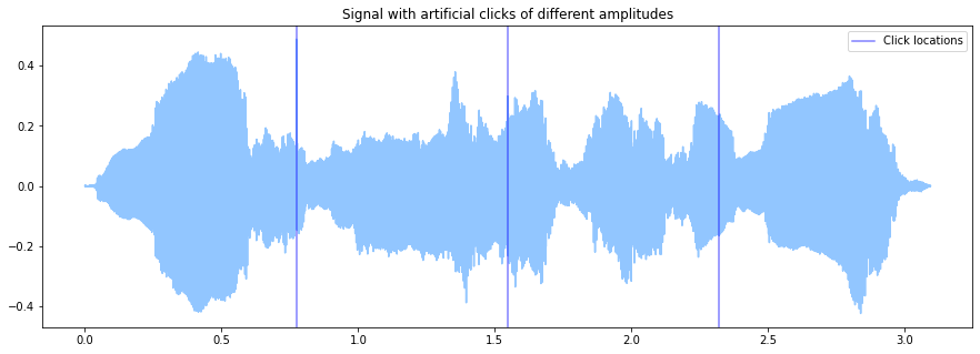

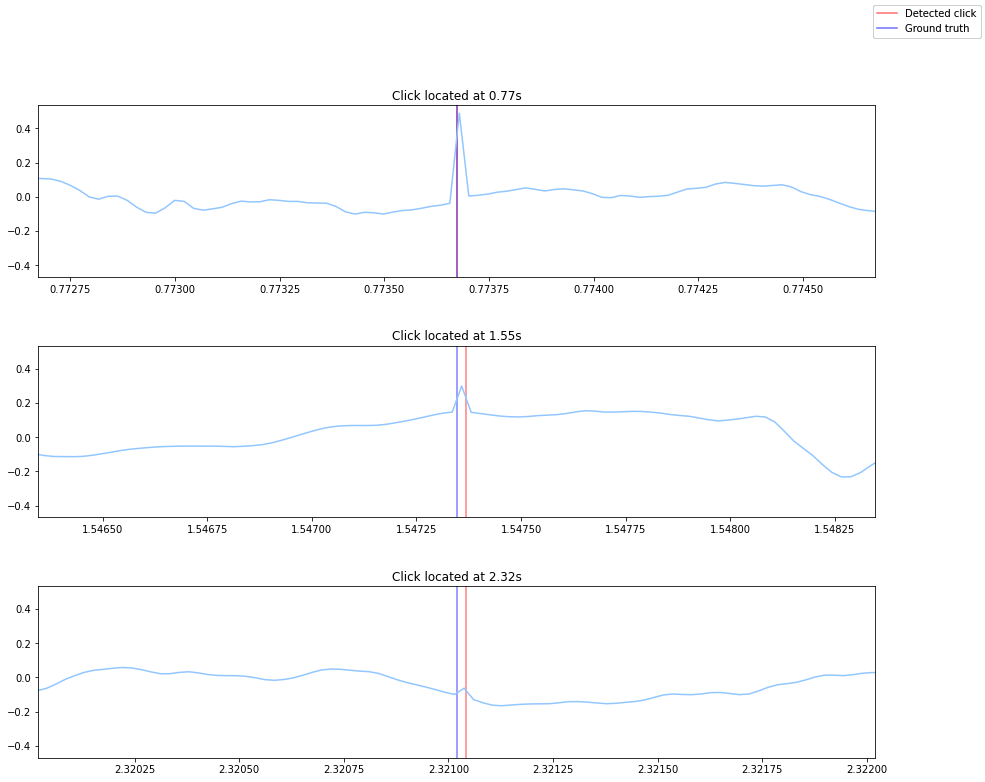
Detection algorithm

The algorithm will output the start and end timestampes of the clicks.

starts, ends = compute(audio)

fig, ax = plt.subplots(len(groundTruth))
plt.subplots_adjust(hspace=.4)
for idx, point in enumerate(groundTruth):
    l1 = ax[idx].axvline(starts[idx], color='red', alpha=.5)
    ax[idx].axvline(ends[idx], color='red', alpha=.5)
    l2 = ax[idx].axvline(point, color='blue', alpha=.5)
    ax[idx].plot(times, audio)
    ax[idx].set_xlim([point-.001, point+.001])
    ax[idx].set_title('Click located at {:.2f}s'.format(point))
    
    
    fig.legend((l1, l2), ('Detected click', 'Ground truth'), 'upper right')

Algorithm parameters

A description of the most relevant parameters of the algorithm

• detectionThreshold = this algorithm features an adaptative threshold obtained from the instant power of each frame. This parameter is a gain factor to adjust the algorithm to different kinds of signals. Typically it should be increased for very "noisy" music as hard rock or electric music. The default value was empirically found to perform well in most of the cases.


• powerEstimationThreshold = after removing the auto-regressive part of the input frames through the LPC filter, the residual is used to compute the detection threshold. This signal is clipped to 'powerEstimationThreshold' times its median as a way to prevent the clicks to have a huge impact in the estimated threshold. This parameter controls how much the residual is clipped.


• order = the order for the LPC. As a rule of thumb, use 2 coefficients for each format on the input signal. However, it was empirically found that modeling more than 5 formats did not improve the clip detection on music.


• silenceThreshold = very low energy frames can have an unexpected shape. This frame can contain very small clicks that are detected by the algorithm but are impossible to hear. Thus, it is better to skip them with a silence threshold.

Summary

Developing more intelligent agents and studying our interaction with them help us better understand human behavior and cognition. The task of building more intelligent machines includes challenges in machine hearing in which we optimize, parse, and detect a relevant feature set. This article provides a high-level summary of the following audio features.

1. Time domain features: windowing techniques, zero-crossing rate (ZCR), characterizing energy using short time energy (STE) and root mean square energy (RMSE), separating harmonic & percussive signals, and beat extraction.
2. Frequency domain features: chroma-related features, tonality based features
3. Spectrum shape based features: spectral centroids, spectral contrast, spectral rolloff, and mel-frequency cepstral coefficients (MFCCs)
4. Using features for analysis: hum, discontinuity, and click detection algorithms

All code and audio samples are available on GitHub @rramnauth2220 with ♥.

References

1. Barchiesi, D., Giannoulis, D., Stowell, D., & Plumbley, M. D. (2015). Acoustic scene classification: Classifying environments from the sounds they produce. IEEE Signal Processing Magazine, 32(3), 16-34. [PDF]
2. Rahmani, M. H., Almasganj, F., & Seyyedsalehi, S. A. (2018). Audio-visual feature fusion via deep neural networks for automatic speech recognition. Digital Signal Processing, 82, 54-63. [PDF]
3. Bachu, R. G., Kopparthi, S., Adapa, B., & Barkana, B. D. (2010). Voiced/unvoiced decision for speech signals based on zero-crossing rate and energy. In Advanced Techniques in Computing Sciences and Software Engineering (pp. 279-282). Springer, Dordrecht. [PDF]
4. Brandt, M., & Bitzer, J. (2014). Automatic Detection of Hum in Audio Signals. Journal of the Audio Engineering Society, 62(9), 584-595.
5. Blue, L., Vargas, L., & Traynor, P. (2018, June). Hello, Is It Me You're Looking For? Differentiating Between Human and Electronic Speakers for Voice Interface Security. In Proceedings of the 11th ACM Conference on Security & Privacy in Wireless and Mobile Networks (pp. 123-133). [PDF]
6. Mühlbauer, R. (2010). Automatic audio defect detection. Bachelorarbeit. Bachelor of Science im Bachelorstudium Informatik, Jonhannes Kepler Universität Linz.
7. Vaseghi, S. V., & Rayner, P. J. W. (1990). Detection and suppression of impulsive noise in speech communication systems. IEE Proceedings I (Communications, Speech and Vision), 137(1), 38-46.
8. Vaseghi, S. V. (2008). Advanced digital signal processing and noise reduction. John Wiley & Sons. Page 355.

Post Tags python essentia librosa audio